Losing customers is costly for every business. But if you understand the who, when, and why of user inactivity, you can diagnose and reduce churn. At Vidora, we help global Fortune 500s improve customer engagement by predicting which users are at risk of churn and why, enabling automated solutions to maximize customer retention. Vidora is constantly exploring new ways to predict and prevent churn. Recently, we’ve focused these efforts on state-of-the-art deep learning techniques.
Background on Recurrent Neural Networks
Deep learning is a not a new technology. However, its practical use has grown dramatically alongside computing power and data availability over the past five years. Two neural network architectures that have shown to be highly effective in sequence modeling tasks are Convolutional Neural Networks (CNNs) and Recurrent Neural Networks (RNNs) [1]. The upshot to leveraging these architectures for churn prediction is their promise of “automatic feature engineering.” The task of identifying and extracting predictive features from raw data has traditionally been handled by data scientists.
However, if implemented correctly, RNNs and CNNs obviate the need for such manual work. This is due to their ability to learn sequential and time-dependent structures inherent in the data. In a previous analysis, we evaluated how CNNs may enhance a business’s ability to retain customers through automated feature engineering and deep learning. In this post, we explore the same question as it pertains to RNNs.
The Importance of Feature Engineering
Before any supervised machine learning problem may be solved, various steps must be taken to prepare raw data for ingestion into a machine learning framework. Of these steps, feature engineering is often the most difficult and time-intensive, but also the most critical to the success of the model [2]. Feature engineering is the process of transforming raw data into more complex structures. These structures represent the data in more predictive ways. The machine learning algorithm then examines these features to find a pattern. That pattern is a mathematical function which signals the risk of churn. The pattern the algorithm finds in sample training data should generalize well enough to predict unknown outputs from unseen inputs.
Modeling Time Dependencies
Different machine learning algorithms take different statistical approaches to finding these patterns. In doing so, many lose the notion of time. Random forests, support vector machines, logistic regressions, and others evaluate all features of each data point in a single step, with each input processed independently of the others [3]. This be computationally inefficient. However, it also may lead to overfitting, because sequences are learned in a fixed manner.
To contextualize each data point relative to the others, time-dependent and sequential structures can be reintroduced to the model through manual feature engineering. For example, time-dependent features which might be engineered to predict churn from user click data include rates of change, aggregate clicks over a trailing window, or sequences of clicks. This “handcrafted” approach, however, has drawbacks — how do we know which transformations will yield the most predictive features and create the most accurate model?
Answering this question can be an expensive process that requires domain knowledge, trial and error, and vast computational resources [2]. To automate and optimize this process would improve Vidora’s ability to predict churn while reducing the time and resources needed. This is where RNNs can help.
RNNs automate the feature engineering process. They do this by learning an internal representation of the data . This representation contains latent features. These latent features can’t be observed directly. They are most useful in generating the desired output. By unearthing which features are most predictive of propensity to churn, RNNs may allow businesses to devise retention strategies.
Why RNNs?

To understand how RNNs are well-suited for engineering features from sequential data, consider neural networks trained via a supervised approach as performing representation learning [4]. Put another way, neural networks provide mathematical rules for learning latent features within the data. In a feedforward network, we accomplish this task in a hierarchical fashion. This means we learn new representations of the data in succession. Each layer distilling latent features will be more and more resolved.
Each layer of the network then learns how to transform the inputs. This occurs via weights, and we ascertain their optimal values (those that get us closest to the expected output) during network training and backpropagation. The last layer of the network typically acts as a linear classifier and uses the learned representations to generate a final output (for our purpose, a probability of churn).
Time Dependency with RNNs
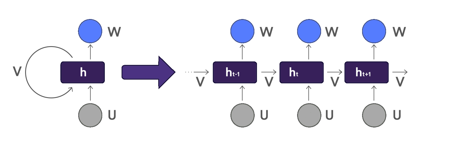
In a RNN, these representations are learned in a temporal fashion, each time step distilling the latent features to be more and more resolved. This notion of time dependency develops at each time step by evolving a hidden state. This equals a sum of (1) weighted input and (2) weighted hidden state from the previous step. We then combine the hidden state with the weighted input at the current time step. You can also think of this hidden state vector as a condensed representation of all the past time step inputs.
Those inputs then take the form of latent features relevant to the task at hand. The optimal weights of the RNN are ascertained via backpropagation through time (BPTT). This is a technique which applies the standard backpropagation algorithm to each time step in the sequence.
Another important difference between traditional feedforward networks and RNNs is weight sharing. While feedforward networks use separate weights for each input feature, RNNs share the same weights across each time step. This not only imposes an additional awareness of time to the network, but also allows the network to better generalize to sequence lengths not seen during training [4].
Conclusions
Our experiments using RNNs to engineer time-dependent features and model churn have shown performance on par with time-agnostic machine learning algorithms using handcrafted features. The results are promising in that they suggest that time-based feature engineering may be automated without sacrificing model performance. These conclusions, however, are not without caveats. Most notably, RNNs are notoriously difficult to train. They are also prone to vanishing gradients, the result of backpropagating errors across many time steps.
However, a variation on the original RNN architecture, Long Short-Term Memory (LSTM), solves this vanishing gradient problem by incorporating additional mathematical operations that modulate past information used in the original RNN [3]. As we iterate on our exploratory efforts and add complexity to the learning architecture, we hope to gain a better understanding of which deep learning algorithms are best. This especially includes the prevalent issue of predicting and minimizing churn.
Citations
[1] Shaojie Bai, J. Zico Kolter: “An Empirical Evaluation of Generic Convolutional and Recurrent Networks for Sequence Modeling”, 2018; [http://arxiv.org/abs/1803.01271 arXiv:1803.01271].
[2] Pedro Domingos: “A few useful things to know about machine learning”, Commun. ACM, 55, pp. 78-87, 2012; [DOI: https://doi.org/10.1145/2347736.2347755]
[3] Zachary C. Lipton, John Berkowitz: “A Critical Review of Recurrent Neural Networks for Sequence Learning”, 2015; [http://arxiv.org/abs/1506.00019 arXiv:1506.00019].
[4] Ian Goodfellow, Yoshua Bengio & Aaron Courville. Deep Learning. MIT Press, 2016, pp. 367-376.


