Can Neural Networks Provide Insight into User Churn?

Introduction

At Vidora, we’ve been exploring the potential for learning techniques such as convolutional networks and autoencoders to improve our understanding of why users churn. Typically, we see neural networks  as “black box” models. This means that they provide high accuracy but very little interpretability. Unfortunately, a model that cannot be interpreted is of little use for Vidora, given our focus on preventing churn, not just predicting it. A prediction can only go so far, but understanding why a user is churning allows us to ultimately provide automated mechanisms to prevent them from doing so. Vidora’s Intelligence APIs automate engagement through customer touchpoints. This means that they reduce churn, due to this understanding of why churn occurs.

In the course of our work at Vidora, we have found that predicting churn is often much easier than automatically preventing it. Often times, simply looking at a user’s activity and training basic models on that activity can provide a good understanding of which users will ultimately churn (the problem of churn prediction and how effective simple machine learning models can be is largely a function of the problem domain).

Our Goal

For these reasons, we’ve been emphasizing the ability to understand what the models have learned, and our goal in this investigation is to explore how neural networks can be used to understand user churn.

In this analysis, we investigated the weights of a trained convolutional network and used autoencoders to visualize diverging patterns of behavior between churned and active groups. We reduced the complexity of the problem significantly, in order to deeply understand how neural networks can provide insights into business questions. In some ways, the networks are toy examples – but they do provide some insights into how neural networks can be used to not only predict but understand user churn.

Convolutional Neural Networks

Convolutional neural networks and autoencoders have been described as an effective method for churn prediction and understanding in the literature [1].

Introducing Convolutional Neural Networks

Convolutional neural networks (CNNs) are a specific type of neural network that have seen exceptional success in image recognition over the past five years. CNNs are unique because they make use of convolutional layers, which are neural network layers that use convolutions. Convolution is an operation in which a filter function is applied to a signal function to produce a third related function.

Convolution has been extremely useful in computer vision for decades. In this context, both the signal function and filter function are matrices. When certain filter matrices convolve over an input image matrix, we see interesting results such as edge detection. In convolutional neural networks, each convolutional layer contains at least one filter. In deep networks, there may be hundreds of different filters. These filters update as the network trains.

Work done with CNNs

The majority of work with CNNs has been in the field of image recognition. However, they work excellently for the problem of churn prediction and prevention as well. First, they work well for temporal data – the convolution operation helps in fields heavily based in time series, such as signal processing. Traditional machine learning models struggle to model and leverage temporal information directly. By using CNNs, we can represent each user as a time series of behavioral events, rather than an aggregation over an arbitrary window. Typically when predicting user churn we have at our disposal a time series of events.

In addition to their suitability for time series, CNNs are significantly more interpretable than other neural network architectures. In fact, we often describe convolutional filters in the network  as “feature extractors”. This is because they identify the most important features to pull from an input before making a prediction. After a model has been trained, the filters can be studied to understand what features they are looking for. We show examples of trained filters from an image recognition model below. The network learns to extract the features that are most unique to the different classes it needs to identify.

Autoencoders

Autoencoders are a special type of neural network with inputs that are equal to the outputs. Put another way, an autoencoder is a network that attempts to learn the identity function. When the number of hidden units is equal to or larger than the dimensionality of the inputs, this is a trivial task. However, when the number of hidden units is small, the network has to learn a compressed representation of the data. Similar to other dimensionality reduction techniques such as PCA and ICA, autoencoders can reveal interesting structure about the input data. In this way, they can also be used as “feature extractors”.  The main difference in autoencoders compared to other techniques is that they have no linearity constraint. Here is a simple autoencoder network below.

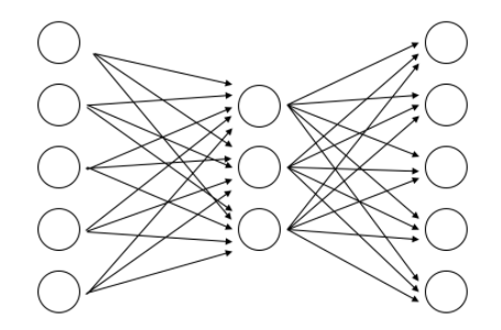
This network learns to compress input vectors from length 5 to length 3 and then decompress to an output that matches the input as closely as possible.

To understand what the autoencoder has learned, it may be visualized. To do so, we can calculate the input that maximally activates each hidden unit of the network. This input may be thought of as the feature the hidden unit is attempting to represent. Then, you can generalize an image by treating each value of the feature as a pixel intensity.

Data

Data came from web logs for a period of one month. We chose three features and aggregated them per day for each user. This included total clicks, total plays, and total events. We limited data to only three features in order to keep the model as interpretable as possible. The resulting feature set was a 31×3 matrix for each user – three feature values for each day of the month. We defined churn as a user being completely inactive in the following month. After extracting information for the entire user base, we took a subsample in order to keep the data at a manageable size and allow for fast iteration in experimentation.

Model Architecture

We used an extremely simple architecture for the convolutional network. This was also to maximize interpretability prior to running on a larger set of data. We employed two convolutional layers. And each had a single filter. Filters were one dimensional so as to not convolve over both time and features at the same time. The first filter is 31×1. This filter convolves over the entire time period using the same set of weights for each feature. The next filter is 3×1. This filter convolves over the three features. Because the filters are the same length as their input, you can think of them as computing a weighted sum.

Essentially, we first compute a weighted sum over time, resulting in a single value for each feature. Then, we calculate a second weighted sum over the three features. We get a final result – and this is a scalar value which is fed through the sigmoid function in order to produce a final probability. Here is a visual representation below.

Experimental Results: Filter Weights from Model 1

We trained the CNN on our dataset ten separate times with different weight initializations. Vidora did this in order to ensure that the weights always converged to similar values. We then extracted the filter weights were from the model. First, we looked at the weight in the first filter, which convolves over time. See this shown below.

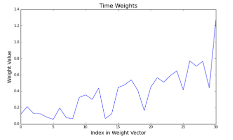
This shows the value of the weight on the y axis, with its position in the weight vector on the x axis. Higher indices correspond to more recent events. It can be seen clearly that the network has learned that more recent activity is more predictive than past activity, even only over the time period of one month. This type of weighting was observed in all models trained.

Experimental Results: Weights Learned in the 1×3 filter

Next, we looked at the weights learned in the 1×3 filter. These can be thought of as weights being placed on each feature, with higher weights meaning a more predictive feature. A plot showing these weights is shown below.

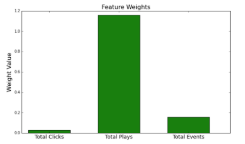
The network has learned that total plays is far more predictive than either of the other two features. Although this is not surprising, it’s interesting to note that total clicks is almost useless in making predictions. With just these three features available, our client should optimize aggressively for plays and not care as much about metrics like CTR.

Next, the customer base was split into active and churned customers and a 3 hidden unit autoencoder was trained on each cohort. The input images that maximize each hidden unit were produced for both autoencoders, three images for each, resulting in a total of six images. The images produced for active and churned users are shown below. In these images, darker shades correspond to higher activity. As in the input matrices to the convolutional network, the rows are days of the month while the columns are the three different features.

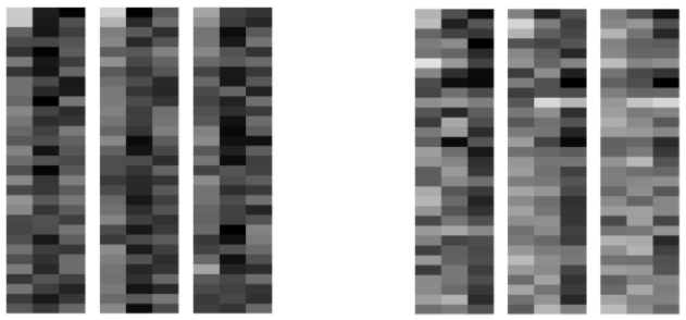
You can draw similar conclusions from the weight analysis of the CNN. There is significantly activity in general in the active users. This is especially true for total plays. The active users show solid play activity consistently throughout the month, while churned user show a much lighter amount of plays. You can see some particularly interesting activity in the first churned image. This image appears to represent a user who starts off with a relatively high amount of plays, but fades out over the course of the month.

Conclusions and Further Work

Both convolutional neural networks and autoencoders offer promise in furthering our understanding of churn, and providing guidance towards the best steps businesses can take to reduce it. Moving forward, we will  introduce significantly more features to the model in order see if it is possible to identify more complex patterns of behavior that are associated with churn. In particular, we are interested in complex temporal dynamics. As we slowly add complexity to the convolutional architecture, we hope to learn more from the filters that each network learns, and gain an ever deeper understanding of how to automatically decrease churn.

Citations

1. Wangperawong, Artit, Cyrille Brun, Olav Laudy, and Rujikorn Pavasuthipaisit. “Churn analysis using deep convolutional neural networks and autoencoders.” ArXiv (2016): n. pag. 18 Apr. 2016. Web.
2. Zeiler, Matthew D., and Rob Fergus. “Visualizing and Understanding Convolutional Networks.” Computer Vision – ECCV 2014 Lecture Notes in Computer Science (2014): 818-33. Web.